After the visa interface is installed on the RPi, through python's pyvisa and pyvisa-py, we can begin to interface with instruments.

The full python script file is located at: RPi_MSO_source_code.py.

Part of the code captures the screen off of the oscilloscope and saves it to a png file: 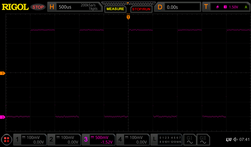where a straight TTL signal is fed into channel 3 and the waveform is displayed in purple.

Let's highlight the important code from the above source file that configured the oscilloscope, captured the waveform, displayed it, and then copied the png file to the host RPi computer. First initialize the script file, import modules, and initialize communications with the oscilloscope:

#!/usr/bin/env python3
# -*- coding: utf-8 -*-
import os#, sys
import psycopg2, psycopg2.extras
from re import compile as re_compile
from sys import argv
from datetime import datetime
from time import sleep
import pyvisa

visa = pyvisa.ResourceManager("@py")
mso = visa.open_resource('TCPIP::192.168.0.222::INSTR')
print(mso.query('*idn?').replace('\n', ''))

mso.write('*rst') #resets the scope to factory defaults.  like pressing "Default" on the front panel.
sleep(5)
#the rest configures the scope to begin acquisition.
mso.write(':channel1:display off; :channel2:display off; :channel3:display on; :channel4:display off')
mso.write(':timebase:scale 500e-6')
mso.write(':display:type dots')
mso.write(':channel3:impedance omeg; :channel3:scale 0.5; :channel3:offset -1.52')
mso.write(':trigger:edge:source channel3; :trigger:mode edge; :trigger:edge:level 1.5')
mso.write(f':acquire:type normal; :acquire:mdepth {memory_depth}')
sleep(1)
mso.write(':single') #command the scope to acquire a single waveform.
mso.write(':system:key:press moff')
sleep(2)

#command the scope to perform a screen capture and transfer that binary data to the host computer and save it as a png file.
print(mso.query(':save:image:type?'))
filename = f'{home_folder}MSO_SC_{filename_id}.png'
r = mso.query_binary_values(':DISPLAY:DATA? ON,0,PNG', datatype='B')
with open(filename, 'wb') as f:
	f.write(bytearray(r))
	f.close()

where the MSO8000 SCPI Programmers Guide can be found on Rigol's website.

All of that works well and fine and screen captures give us that 'ah ha' moment, but there is no data to transfer and analyze in a screen capture. Although, there are some subtleties there, like binary transfer, which will become important soon, we ultimately will need to transfer voltage and timing raw data from the scope, store in in PostGreSQL, evaluate and analyze that data, and finally, draw conclusions from the analysis.

Besides configuring and commanding the oscilloscope, the most important aspect of science is accurately collect and store the data of our experiment. We can easily acquire and transfer a very large string of "floating-point scientifically-notated exponentially-formatted big string of voltages" directly from the oscilloscope, but that is a huge amount of data to transfer and store later in our database. Ultimately, we'll want to minimize the data packet sizes and this will be done with transferring raw bytes from the oscilloscope. Those raw bytes can also be stored directly in a BLOB field in PostGreSQL.

Let's first grab the "floating-point scientifically-notated exponentially-formatted big string of voltages" which will be used to verify our values when we convert the byte voltages to real voltages.

#bos...query for binary the ascii true voltage way
mso.write(f':waveform:source channel{channel}; :waveform:mode raw; :waveform:format ascii; :waveform:points {memory_depth}')
preamble = mso.query(':waveform:preamble?').replace('\n', '').split(',')
print('preamble:', preamble, 'channel:', mso.query(':waveform:source?').replace('\n', ''))
data = mso.query(':waveform:data?')
#print(data, 'number of points:', len(data), 'type:', type(data))
if (preamble[0] == '2'): #ascii returned from mso
	if (data[0] != '#'):
		raise Exception('mso returned invalid ascii list')
	header_length = str_to_int(data[1])
	datasize = str_to_int(data[2:header_length+2])
	lst = data[header_length+2:].replace('\n', '')[:-1].split(',')
	lst = ascii_raw = [str_to_float(v) for v in lst]
	#print(f'\n"{datasize}"\n"{lst}"')
	print(lst, '\nnumber of points:', len(lst), 'type:', type(lst), type(lst[0]))
	x = histogram(lst)
	print(x, len(x), sum([v for k,v in x.items()]))
#eos...query for binary the ascii true voltage way

The list of "floating-point scientifically-notated exponentially-formatted big string of voltages" is now on the console screen for our comparison later on. Now let's grab the byte stream of voltages, which is only 8-bit long for each voltage, hence very small in size. In other words, 10k data points is only 10KB, and not, almost 1MB of the "floating-point scientifically-notated exponentially-formatted big string of voltages".

#bos...query for binary the raw way
mso.write(f':waveform:source channel{channel}; :waveform:mode raw; :waveform:format byte; :waveform:points {memory_depth}')
preamble = mso.query(':waveform:preamble?').replace('\n', '').split(',')
print('preamble:', preamble, 'channel:', mso.query(':waveform:source?').replace('\n', ''))
mso.write(':waveform:data?')
data = mso.read_raw()
print(data, len(data))
if (preamble[0] == '0'): #byte returned from mso
	print(data[1])
	if (data[0] != 35): #the ascii character code for '#'
		raise Exception('mso returned invalid byte list')
	header_length = data[1] - 48 #if the "9" in the 2nd index then data[1] return 57, the ascii character code for '9'
	datasize = str_to_int(data[2:header_length+2].decode('utf8'))
	print(header_length, '%s' % datasize)
	lst = data[header_length+2:-1]
	print(lst, '\nnumber of points:', len(lst), 'type:', type(lst), type(lst[0]))
	x = histogram(lst)
	print(x, len(x), sum([v for k,v in x.items()]))
#eos...query for binary the raw way

PyVisa can grab the data stream in a raw way, as above, or it also has a nice "query_binary_values()" function that does a lot of work for us. So, before moving on to converting bytes to voltages, its good to test the PyVisa "query_binary_values()" function and make sure it matches the byte voltages of the latter code.

#bos...query for binary the visa way
data = mso.query_binary_values(':waveform:data?', datatype='B')
print(data, len(data))
x = histogram(data)
print(x, len(x), sum([v for k,v in x.items()]))
#eos...query for binary the visa way

where the two byte streams match exactly and which simply proves the PyVisa "query_binary_values()" function reliably works for us and minimizes our code in our calling application.

And now let's convert our byte stream into a list of real voltages.

yincrement, yorigin, yreference = str_to_float(preamble[7]), str_to_int(preamble[8]), str_to_int(preamble[9])
print(yincrement, yorigin, yreference)
ascii = ascii_converted_from_bytes = [(b-yorigin-yreference)*yincrement for b in data] #this is the conversion from byte to real voltages
x = histogram(ascii)
print(x, len(x), sum([v for k,v in x.items()]))

Once the program is run, you'll see that the converted voltages match the original voltages to within 5 significant figures. The differences are probably the difference between the on-board computing of the oscilloscope and python themselves.

The following code is a rough hack to output the two voltages to a csv file for quick and dirty analysis in Excel. My output is here: MSO_DATA_CHANNEL3_1.csv.

xincrement, xorigin, xreference = str_to_float(preamble[4]), str_to_float(preamble[5]), str_to_float(preamble[6])
print(xincrement, xorigin, xreference)
s = ''
for i, (ar, ac) in enumerate(zip(ascii_raw, ascii_converted_from_bytes)):
	s += f'{i*xincrement+xorigin+xreference}\t{ar}\t{ac}\n'
with open(f'{home_folder}MSO_DATA_CHANNEL{channel}_{filename_id}.csv', 'w') as f:
	f.write(s)
	f.close()

where the plot for my data is: 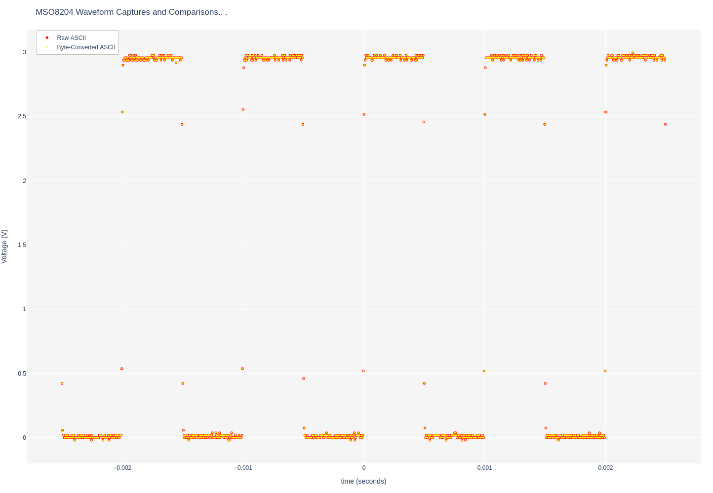where if you click on the plot and zoom into the plot, you'll see that every diamond precisely corresponds with every circle. Meaning, the byte-converted voltages coincide with the oscilloscope's voltages.

In conclusion, this worthy endeavor of using a $80 RPi computer to control and acquire data from modern expensive digital oscilloscopes with the mindfulness of minimizing transfer and storage data sizes of raw data can only lead to efficient and effective instrumentation.

UPDATE

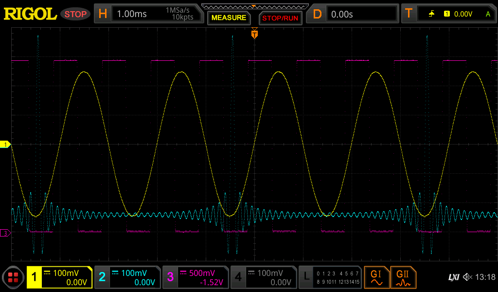
Once all of the above was complete, it was fairly easy to embed the code into a single object. This centralized the code and cleaned up the calling application. With only about a dozen lines in the calling application, the following screen capture was produced: with the corresponding waveforms producing: 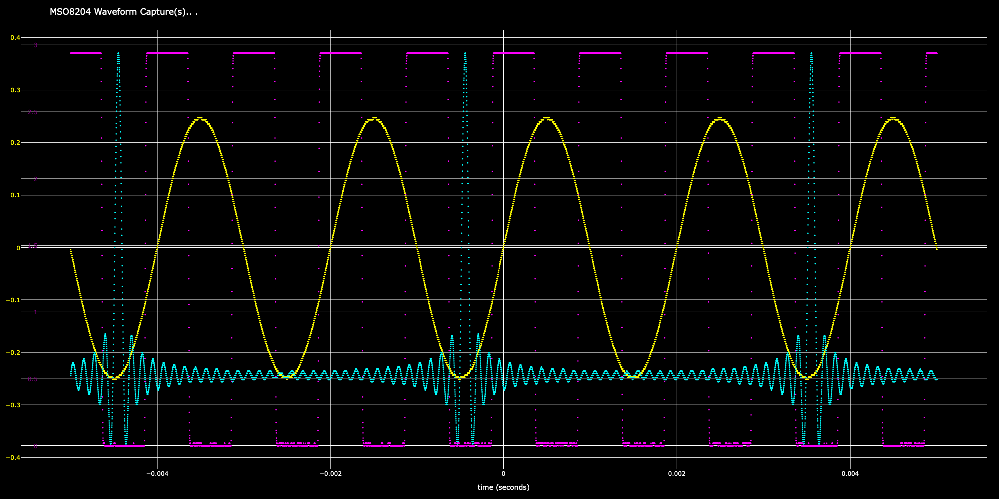which is a png generated with plotly plotting library in a web browser.