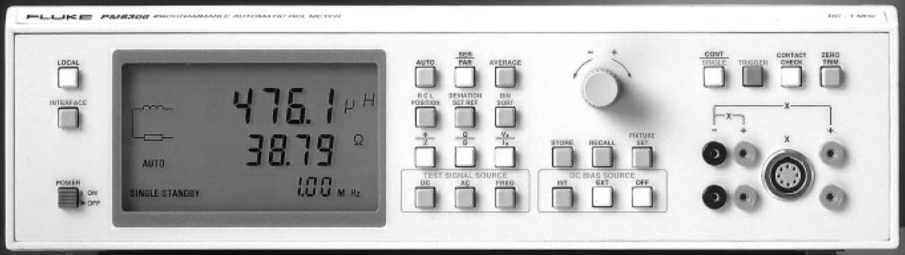
The front panel looks like: and where you'll notice 6 test ports at the bottom right of the front panel: 2 vertical black on the left of that section, and 4 vertical in red just outside the connector port.

I want to understand exactly how the 4-wire kelvin testing works, for it will provide accurate impedance, Z = X_r - jX_i, measurements to within 1% precision. The imaginary X_i term leads to the capacitance via, X_i = (2 π f C)^-1, where f is the frequency in Hertz (Hz) and C is the capacitance in Farads (F).

With the unit off, measuring the resistances of the ports indicate to me that the two "drive high(+)", in red, and the two "sense high(+)", also in red, are the same ports. They are only extensions of each other. The resistance between both top and bottom red ports is 200kΩ, as well as the for the two black ports, "drive low(-)" and "sense low(-)". The resistance between the two top red and black ports is 2MΩ and the two bottom red and black ports is 2.4MΩ. And the diagonal red and black ports seems to have the 200kΩ added to the latter. Also, similar resistances are measured on the 4-terminals of the PM9540/BAN test accessory. In which the 4-terminals are labeled, "Drive(+)" and "Sense(+)" both red, and "Drive(-)" and "Sense(-)" both black.

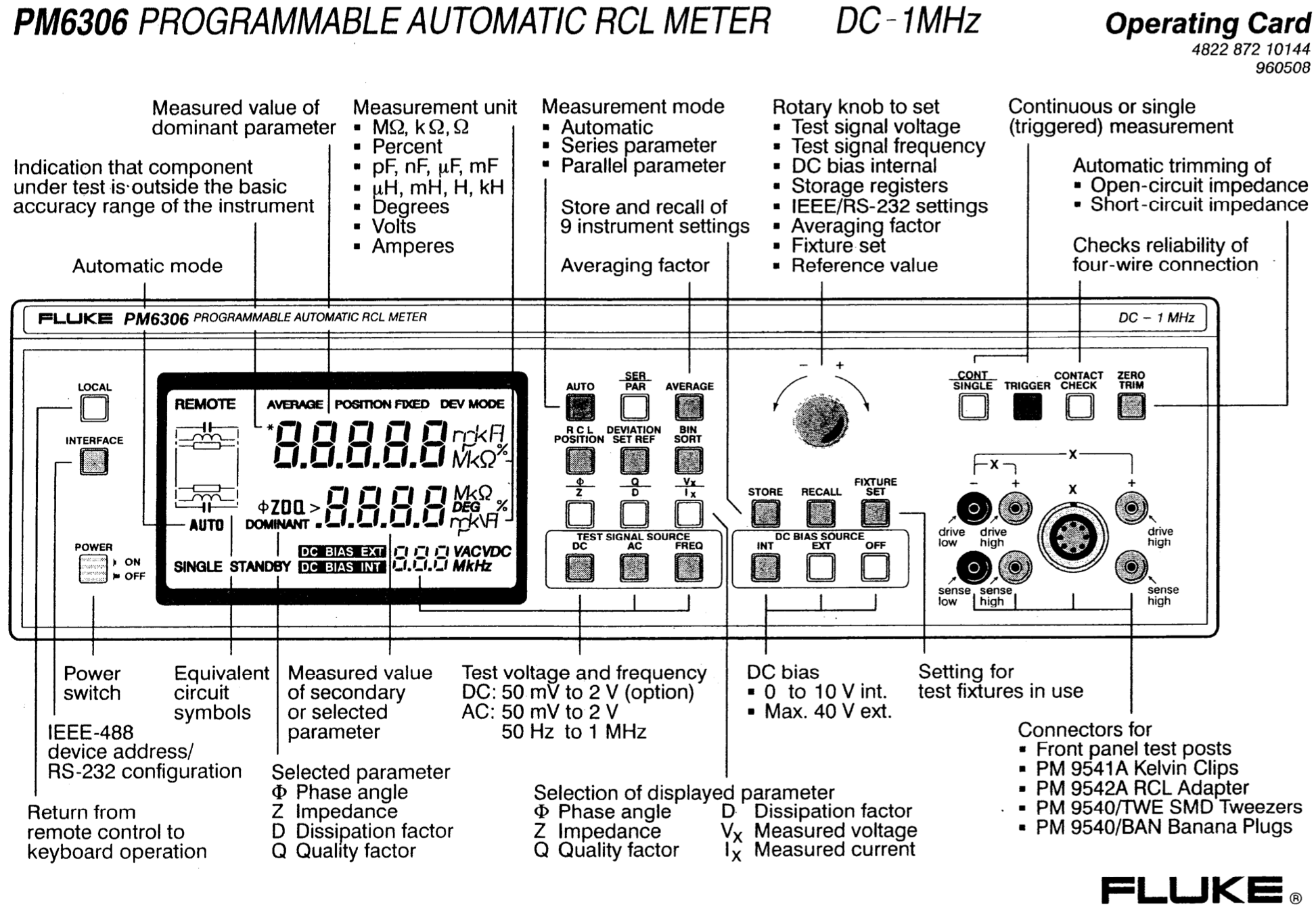
I then connected the 4-terminals to the oscilloscope to view the signal generations and captured them at 50, 1K, and 1MHz. The screen shots follow, first at 50Hz: then at 1KHz: 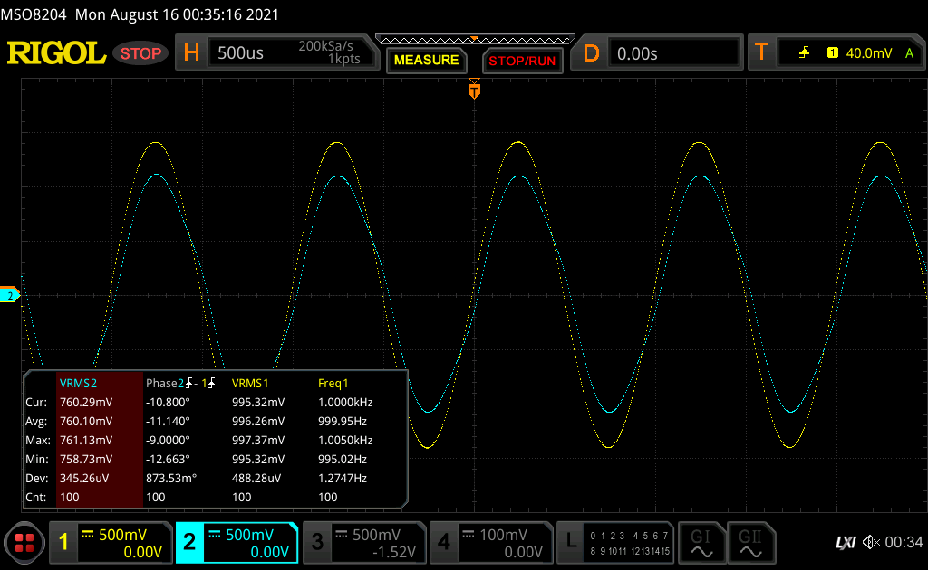and finally at 1MHz: where Channel 1, in yellow, was the "Drive High(+)" to center pin on the coaxial cable with "Drive Low(-)" on shield, and Channel 2, in cyan, was the "Sense High(+)" on center and "Sense Low(-)" on shield. The V_rms measurements were verified on a Fluke 79 DMM.

The above roughly characterizes the electrical properties of the RCL meter. The next step is to use the meter to characterize standard capacitors, make sure the measured capacitance from the meter matches the specifications of the capacitor under test, and develope an impedance spectrum or profile from 50 Hz to 1 MHz of the standard capacitors in order to use as calibration and targets when building an impedance spectrometer using function generators, lock-in amplifiers, and oscilloscopes.

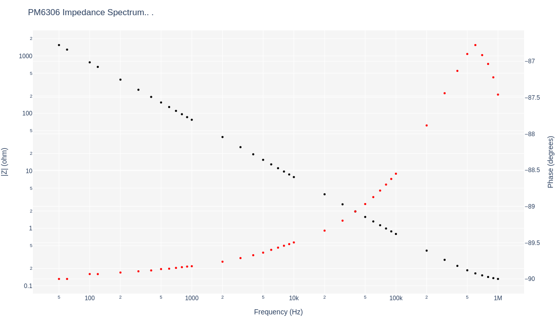
Connecting the Raspberry Pi host and writing a Python program to scan the frequencies and retrieve the meter's measurements, with averaging, to retrieve the complex impedance spectrum yielded, for example: and its corresponding capacitance spectrum: 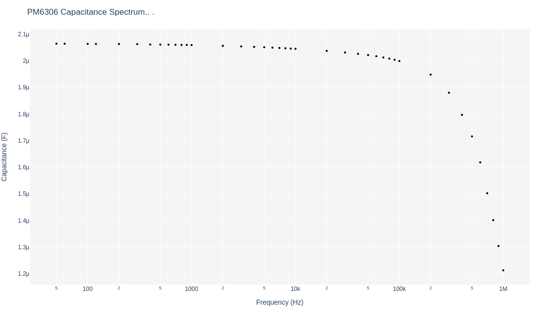for a 2µF axial capacitor. The measured capacitance closely matches the 2µF specification of the capacitor to about 200 KHz.

Ideal vacuum or air capacitors do not have dielectric material sandwiched between the conductive plates, therefore, the above standard capacitor does have a dielectric material as evidence in the phase deviating from -90°. Real or dielectric capacitors will suffer energy losses which are regarded as resistors in series with the capacitive plates. The resistive nature at any particular frequency of a capacitor will exhibit a real component in the complex impedance as X_r, as above. The more resistive the capacitor, the more the phase will measure towards zero. The above capacitor exhibits a maximum phase of 86.7° at 600 KHz.

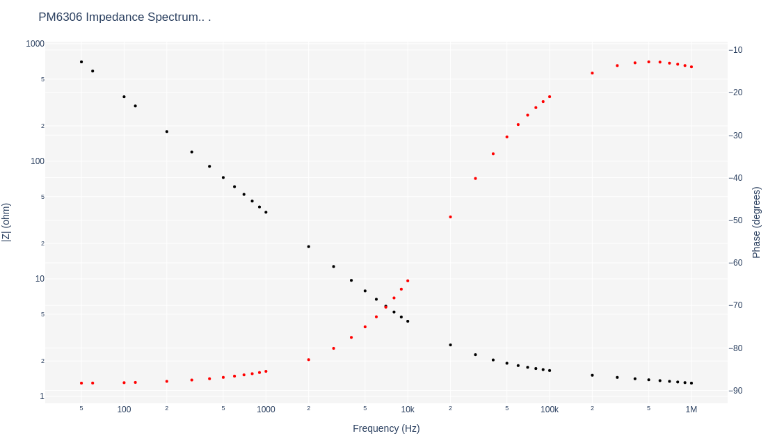
Much more dramatic losses are shown by another capacitor as shown by: and its corresponding capacitance spectrum: 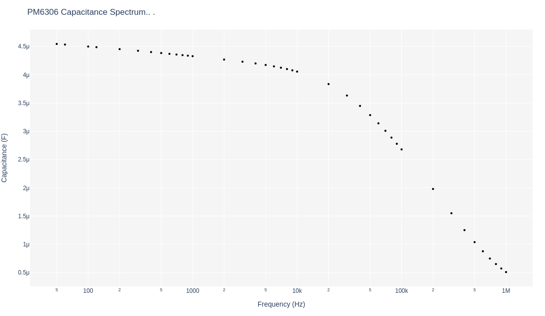where the capacitance below 40 KHz of 4 µF closely matches its specifications and at higher frequencies, the dielectric material is lossy, resistive which the phase reaching a maximum of -12.8° reflects those loss. The point being ultimately, is to match these impedance and capacitance spectra in the proposed instruments to be built.

The PM6306 is a top of the line model valued currently at around $2,200 U.S.D. It has a rather basic remote interface command structure in which after triggering a measurement, the host can only request resistance, capacitance, inductance, impedance magnitude, and phase. And the host must ask these separately for if packaged as a single query and a zero is returned on any one of those the subsequent queries, a null is returned on the rest of the queries. Also the PM6306 does not have internal averaging so to average over a set, the host computer must individually trigger each measurement and iterate until the number of counts is reached. Nonetheless, the PM6306 does not allow for direct acquisition of the complex impedance, but only through individual query of resistance, capacitance, and inductance is complex impedance derived on the host computer via:

impedances.append(complex(R, ((2*pi*f*L) - (1/(2*pi*f*C) if (C != 0) else 0.))))

or via:

impedances.append(complex(Z*cos(pi*phase/180.), Z*sin(pi*phase/180.))

where the former was chosen as the standard and all impedances and capacitances were vigorously cross verified with other native measurements of the PM6306. The complex impedance along with the frequency was ultimately stored in the database for later graphing and analysis.

Johanson manufactures these little piston air trimming capacitors that look like:
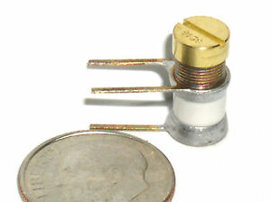
where its screw head allows tuning of the capacitance by screw turns.

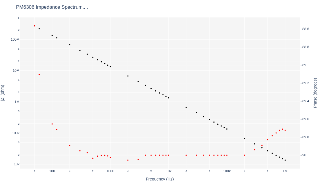
The PM6306 RCL meter produced the below impedance and capacitive spectra for the Johanson 1518 1 to 10 pF capacitor tuned to minimal plate separation: with the respective capacitive spectrum of: 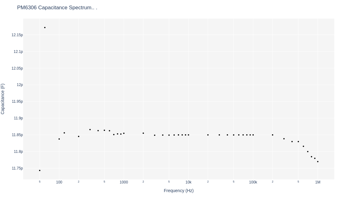where the magnitude of impedance is clearly a log-log relationship, the phases are all around -90° and within 1.5°, and the capacitances are at an average of 11.85 pF and within 0.4 pF of each other throughout the entire frequency range. An excellent example of an ideal capacitor with very little loss and verified at the range of the specifications of the capacitor itself. I've order the Johanson 5601 air trimmer which has a range of 1 to 30 pF and will present its spectra upon its receipt.

A custom sample holder was created in much of the same way as the Johanson trimming capacitors. The custom holder is a parallel plate air capacitor with a 2.5 inch diameter, a guard ring, and the separation between the plates is adjusted using shims. Its impedance and capacitive profiles look like: with its associated capacitive spectrum: where the custom sample holder exceeds the frequency profile of the Johanson capacitors with even less loss at only 0.5° phase range and all capacitances within 3 pF of each other.

At this point, its time to develope the impedance spectrometers using function generators, lock-in amplifiers, and oscilloscopes and reproduce the above PM6303 profiles with the same capacitors as reported above. Besides developing the very slow step-by-step incrementing frequencies in the frequency domain, I also plan on developing time-domain pulsed spectrometers using the Rigol 2 GHz oscilloscope and convert those into the time-domain using Fourier transforms. All these techniques are well published, but dreaming and theorizing are very different then actual physical verifiable results.